My first paper
Today, my first paper - has been released in preprint on the arXiv: Hyperboloidal method for frequency-domain self-force calculations
You can read the paper for free on the arXiv here.
It's new paper day!
At long last, my first paper has been released!
We present a new, alternative hyperboloidal method for for frequency-domain self-force calculations.
Let me briefly introduce you to this new approach.
We consider a scalar field toy-model to demonstrate our approach. This simplified model allows us to understand the problems one might encounter when considering the more mathematically complex, but inherently similar, gravitational problem. It captures all the essential features of self-force calculations while avoiding subtle technical issues in the gravitational case, such as gauge choices.
In general, the frequency domain wave-equations in the self-force problem have the following form for a single scalar field.
In the paper we detail the specific form of this second-order differential operator and the different types of source one can encounter:
Distributional
Worldtube
Unbounded Support
Sources with unbounded support arise in various recent self-force calculations. They appear in second-order gravitational self-force calculations where a contribution to the source for the second-order metric perturbation comes from the second-order Einstein tensor, which is computed from quadratic contributions of the first-order metric perturbation and its derivatives. The two-timescale approach to second-order calculations introduces “slow-time derivatives” of the first order metric perturbation and the calculation of these also introduces these type of source terms.
Traditional frequency domain approaches employ the variation of parameters method and compute the perturbation on standard time slices. The physical boundary conditions are typically specified on $t = \text{constant}$ hypersurfaces that intersect the bifurcation horizon at $r = 2M$ and at spatial infinity as $r$ goes to infinity. The boundary conditions pick the retarded solution whose energy radiates towards the black hole or to infinity.
Practically, however, boundary data is prescribed with asymptotic expansions in order to obtain a solution with the correct behaviour towards the black hole horizon and spatial infinity. This is because one has to find solutions over a finite grid whilst theoretically, the solutions are over an infinite domain.
This approach has been very successful, but boundary conditions calculations can be problematic, and the approach is not well suited to unbounded sources that extend throughout the spacetime.
Our paper develops a more favourable, geometric approach building on the work of Freidrich, Andersson, Schmidt and Zenginoglu for hyperboloidal methods in black hole spacetimes. Avoiding the standard prescription of modelling our perturbations on Cauchy (time) slices, we choose an alternative hyperboloidal foliation with compactification.
Hyperboloidal surfaces are spacelike surfaces that behave like a spacetime hyperboloid near null horizons.
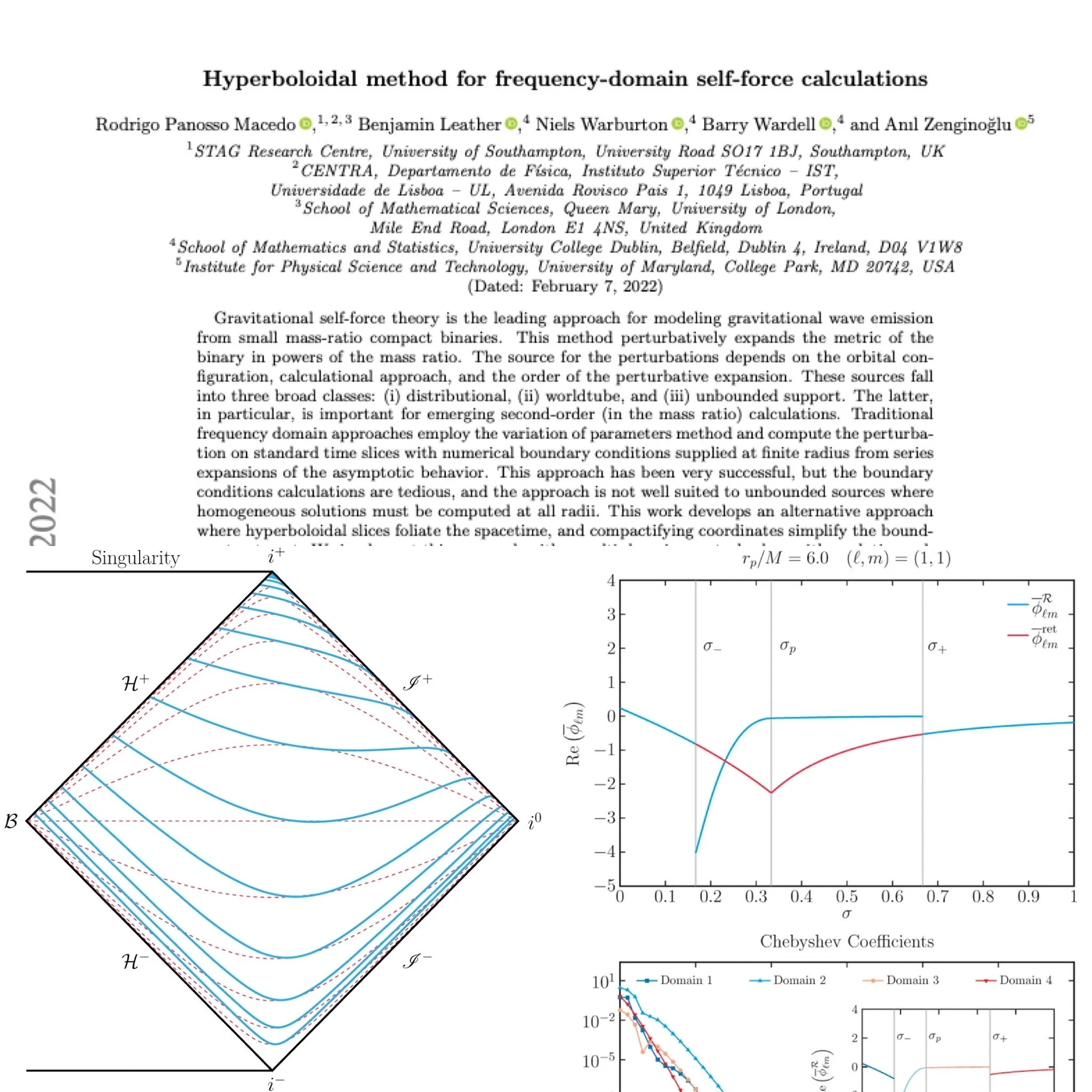
Hyperboloidal coordinates foliate the future event horizon instead of intersecting at the bifurcation sphere and they foliate future null infinity instead of intersecting at spatial infinity. You can see this in the Carter-Penrose diagram below. Thin, red dashed lines depict standard Schwarzschild exterior time surfaces whilst the thick, blue lines depict hyperboloidal time surfaces, where $\tau$ is constant. These coordinates provide a smooth foliation on the full exterior domain which means that both the horizon and null infinity can be included in the computational domain.
This removes the troublesome need to derive boundary conditions from Frobenius or asymptotic series expansions. In fact, if one constructs the hyperboloidal coordinates in such a way that the hyperboloidal time hypersurfaces extend between the black-hole horizon and future null-infinity then the boundary conditions become trivial.
Here, we follow and work in the so-called minimal gauge. Specifically, the transformation between the original Schwarzschild coordinates and the hyperboloidal coordinates reads as below. Here $\tau$ is our hyperboloidal time and not to be confused with proper time.
$H$ is the height function given by the following expression in terms of the new coordinate $\sigma$. Thus, along $\tau = \text{constant}$, scri-plus is located at $\sigma = 0$ and the black-hole horizon is at $\sigma = 1$.
For regularity of the transformed equations, the asymptotic fall-off behaviour of the unknown field must be taken into account. In the frequency domain, this translates to a rescaling of the following form. The hyperboloidal field satisfies a new equation with the operator and source related to the originals via the following.
The conformal factor, $\Omega$, accounts for the scalar field’s fall-off behaviour $\sim 1/r$, whereas the exponential term naturally arises from the Fourier factor when the time transformation is taken into account. In this way, $Z$, automatically incorporates the boundary behaviour via the geometrical interpretation of the height function. Here I give the form of $\boldsymbol{A}$ and the re-scaling factor for our case. This factor would change if the spin-weight of the Teukolsky equation was different.
An important property is that the transformed operator $\boldsymbol{A}$ degenerates at the domain boundaries. In other words, the operator’s principal part, $\alpha_{2}$, vanishes at $\sigma = 0$ and $\sigma = 1$. Thus, the original considerations about in-going/outgoing boundary conditions are re-casted into questions about the underlying solution’s regularity.
In practical terms, due to the vanishing of the coefficient $\alpha_{2}$ at $\sigma = 0$ and $\sigma = 1$, the regularity conditions for a field $\phi$ are given by the following expression. Hence, the boundary conditions follow directly from the equation, and no external data is allowed if one seeks a regular solution.
Put simply, the boundary conditions follow directly from the differential equation. There’s no need to provide data on the grid boundaries because there are no incoming characteristics into the numerical domain.
In the paper we also detail how to transform the scalar field equation for each type of source and also discuss how to further transform the equations for the flux and self-force. This is particularly useful for when calculating fluxes towards null infinity as one can directly read-off values for the radiative flux without the need for extrapolation.
We solve our hyperboloidal equation using a multi-domain spectral method.
For example, our code finds excellent agreement with regions of the parameter space traditionally not suited to perturbative computations, especially towards the weak-field regime of large orbital radius usually covered by the post-Newtonian theory.
First of all, here is a comparison with the $t$-component of the self-force calculated from flux balance laws with a scalar field 4PN expression. The plot on the left is a comparison of the $t$-component of the self-force normalised by the leading PN term.
This plot is the comparison of the parametric-derivative of the same component and it demonstrates the applicability of the method with unbounded support sources that extend throughout the spacetime.
You find similar “slow-time” derivative expressions and calculations in the second-order calculation from the two-timescale approach.
The blue line is a comparison with the leading PN term and each subsequent line are the residuals after subtracting successive PN terms.
Secondly, here are plots of the $\ell$-mode contribution to the regularised $r$-component of the scalar self-force for the mode-sum and effective-source methods. Each line represents a subtraction of analytic regularisation parameters designed to ensure the physical self-force is resolved from the divergent retarded field.
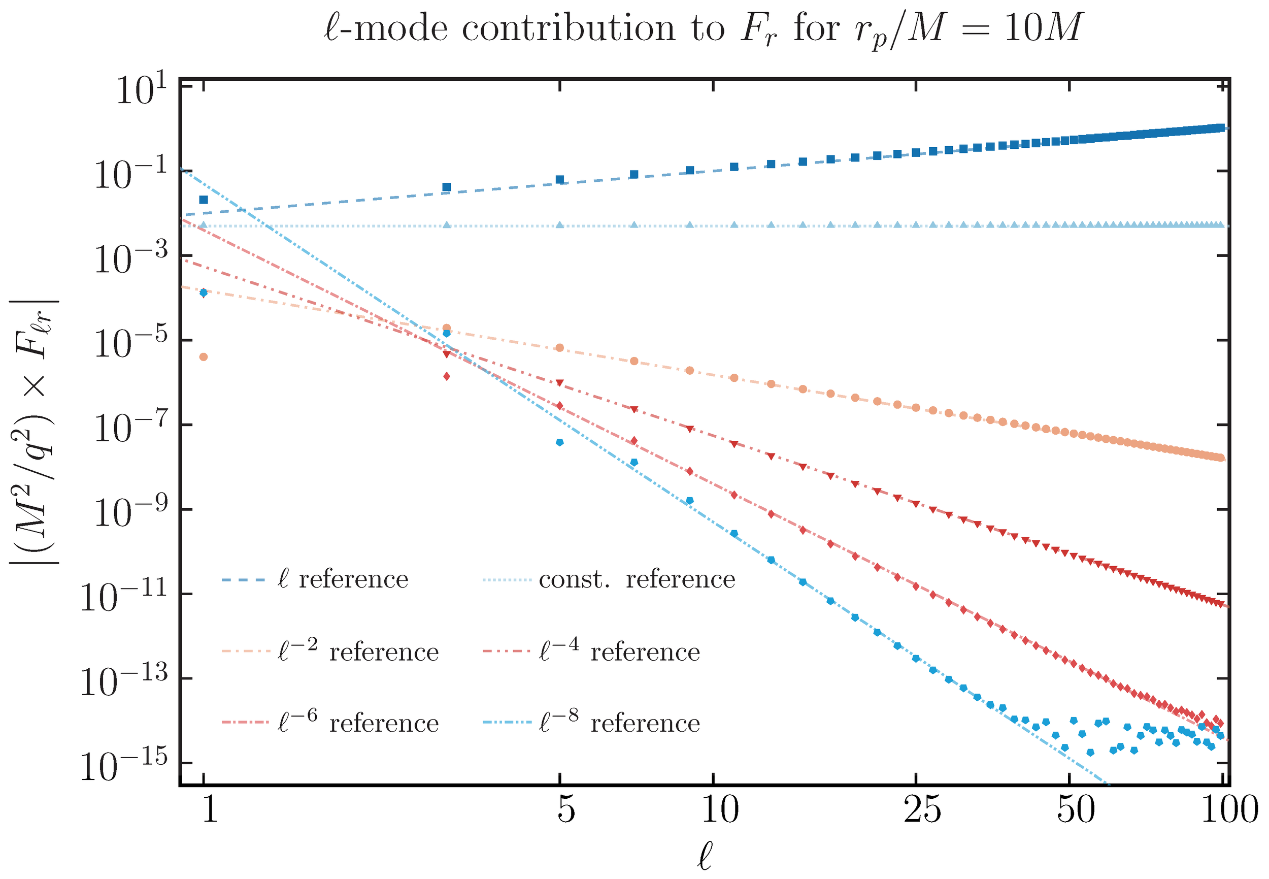
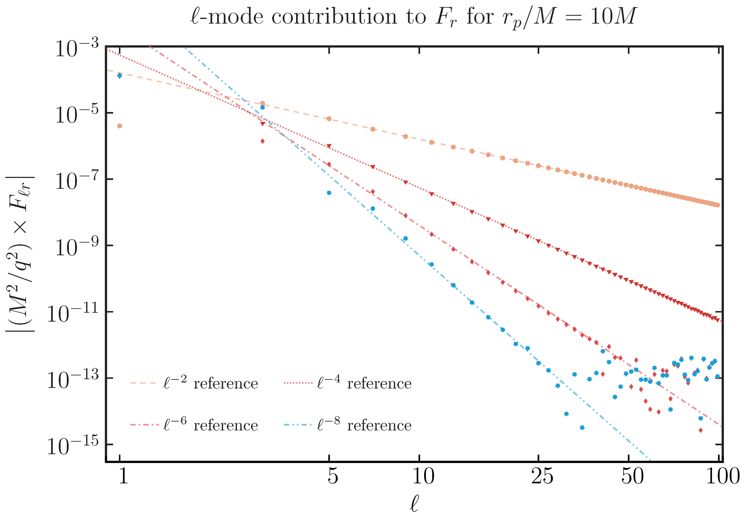
The key thing to note here is that typically one is only practically able to resolve up around $\ell \sim 50$ modes, whilst our spectral hyperboloidal code can quickly and efficiently manage up to $\ell \sim 100$ without too much difficulty for both methods. Even with regularisation parameters, in some cases like close to the light-ring one does indeed require a large $\ell$-mode spectrum.
We are confident the approach we have developed will play a crucial role in future self-force calculations. In fact, we are already seeking to replace the traditional variation of parameters method in our second-order calculation. The main reason for this is the remarkable ability to deal with unbounded support sources like you find in second-order calculations.
This work was done in collaboration with Rodrigo Panesso Macedo, Niels Warburton, Barry Wardell and Anıl Zenginoğlu.
This article was based on a recent seminar I gave (remotely) for the University of Southampton.